Yagel Numbers: the Mersenne × Primorial Grid — Structure, a Lucas–Lehmer-Type Test, and Proven Primes at Scale

Yagel Bar · Revision 2.6 — September 27, 2026 (Revision 2.0: July 2, 2026; Revision 1.0: October 23, 2024)

This is a living document. Revision 1.0 appeared October 23, 2024. The present revision reports the family's structure theory, its deterministic primality criteria, the census of both faces over the original domain, the first forward campaigns (June–July 2026), and the method behind the catalogue of proven primes, whose current contents are published as versioned data releases (§5.2). Corrections carried by this and earlier revisions are collected in the scientific errata at the end, together with a statement of what each claim below does and does not establish.

1. Introduction

Mersenne numbers $M_n=2^n-1$ owe their role in prime searching to two gifts: an algebraic one — a divisor $2^d-1\mid 2^n-1$ for every $d\mid n$, so only prime exponents need testing — and an arithmetic one — the Lucas–Lehmer test, which decides the primality of $M_p$ with one quadratic recurrence modulo $M_p$. It is natural to ask what becomes of these gifts when the sieve idea behind Mersenne numbers ("exclude divisibility by 2") is pushed to its logical extreme.

Fix $k\ge 1$ and let $p_k$ denote the $k$-th prime, $p_{k-1}\mathrm{\#}=\prod _{j<k}{p}_j$ the primorial ($p_0\mathrm{\#}=1$). A Yagel number of order $k$ and exponent $n$ is

$$\begin{array}{}\text{(1)}& Y_k(n)=p_{k-1}\mathrm{\#}\cdot p_k^n-1=2\cdot 3\cdot 5\cdots p_{k-1}\cdot p_k^n-1,k,n\ge 1.\end{array}$$

The construction removes divisibility by every prime up to the base: the primorial coefficient kills the primes below $p_k$, the power $p_k^n$ kills $p_k$ itself (§2.1). Two classical families appear as the boundary of the grid:

• row $k=1$: $Y_1(n)=2^n-1$, the Mersenne numbers;
• column $n=1$: $Y_k(1)=p_k\mathrm{\#}-1$, the primorial numbers, whose primes are the primorial primes studied since Dubner [7] and Caldwell–Gallot [8].

Both "constants" in (1) are dictated by the prime sequence itself; the family has no free parameters and is indexed purely by the lattice point $(k,n)$. The genus is classical: numbers $c\cdot b^n-1$ with fixed coefficient and base have been studied since Lucas, with Riesel ($c\cdot 2^n-1$), Williams ($(b-1)b^n-1$), and their $+1$ mirrors (Proth, Sierpiński, Thabit) as the familiar branches — and we claim nothing beyond that placement. What singles $Y$ out within the genus is that the coefficient is not one of infinitely many arbitrary choices of $c$ but the parameter-free one, $c=p_{k-1}\mathrm{\#}$, coupled to the base $b=p_k$: the specialization with the smallest positive coefficient giving the prescribed congruences for its base (§2.1) and the adjacent integer is fully factored at every cell (§2.3). The result is a natural two-dimensional table whose edges are Mersenne and primorial numbers and whose interior appears not to have been treated as a single object before.

Notation and nomenclature. Following the convention of Lucas sequences and Chebyshev polynomials, we call $Y_k^{-}(n)=p_{k-1}\mathrm{\#}{p}_k^n-1$ the Yagel numbers of the first kind and $Y_k^{+}(n)=p_{k-1}\mathrm{\#}{p}_k^n+1$ the Yagel numbers of the second kind; an unmarked $Y_k(n)$ always means the first kind (the historical default of Revision 1.0). Informally, as in the Cunningham tables' "$-$ side / $+$ side", we speak of the $-1$ and $+1$ faces of the grid around the central column $M=p_{k-1}\mathrm{\#}{p}_k^n$. The second kind has classical edges of its own: its $n=1$ column consists of the Euclid numbers $p_k\mathrm{\#}+1$, and its $k=1$ row is $2^n+1$, prime at most when $n$ is a power of two — the Fermat form (see §4.5).

What is new here, and what is not. Numbers $c{b}^n\pm 1$, their Lucas-type primality tests, and the two edges of the grid are classical (§3 lists the prior art for the test). What this paper introduces is the coupling: the coefficient is not a free parameter but the primorial of every prime below the base, and the base is the next prime — a canonical, parameter-free two-parameter family in which the Mersenne numbers are the first row and the primorial numbers the first column. No name, sequence, or treatment of this family as one object was found in the literature or the OEIS. Everything below is a consequence of the coupling and, to our knowledge, appears here for the first time: the structure theory of the grid (maximal sieve, Proposition 1; no dead cells, Lemma 2; no cheap coverings, Lemma 2′); the test of the interior stated as one family of Chebyshev maps $x\mapsto V_{p_k}(x)$ with the classical Lucas–Lehmer iteration as its first member and a seed valid on every cell (§3); the linear-time reduction in radix $p_k$ (Proposition 4); the first-order statistical account of the census — the Mertens factor, the $k$-free window law (4), and the isoefficiency of searching across rows (§4–5); the census of both faces to 5000 digits, the cells proven prime on both faces, and the large primes of §5; and the integer sequences the grid defines (first primes of each row, and the columns of both faces), prepared for the OEIS.

This paper presents the family from three angles.

Structure (§2). The sieve property is maximal; the interior admits no algebraic factorization in the exponent (a Capelli-type lemma), so every lattice cell is a live candidate — in sharp contrast to the Mersenne row, where composite exponents are disqualified; and both neighbors $Y\pm 1$ of the central point $M=p_{k-1}\mathrm{\#}{p}_k^n$ come fully factored.

A deterministic test (§3). Because $N+1$ is fully factored, the classical Brillhart–Lehmer–Selfridge theory applies to every member. We state and prove the test in its sharpest form for this family: in the one-ladder regime $p_k^n\ge p_{k-1}\mathrm{\#}+2$ (all but finitely many cells of each row), primality of $N=Y_k(n)$ is decided by a single $V$-only Lucas ladder — an $n$-fold iteration of the degree-$p_k$ Chebyshev-type map $V_{p_k}$, seeded at $V_h(P)$. For $k=1$ the map is $V_2(x)=x^2-2$ and the criterion collapses to the Lucas–Lehmer(-Riesel) test verbatim. The cost is about two multiplications per bit, roughly three Fermat tests, and the output is a proof, not a probability. Tests of this kind are classical for the whole $c{b}^n\pm 1$ genus (§3, Prior art); the grid's contribution is structural, not algorithmic — the hypotheses of every such theorem are met by construction at every cell — and, in radix $p_k$, the reduction modulo $Y_k(n)$ is a single multiplication by the primorial (Proposition 4).

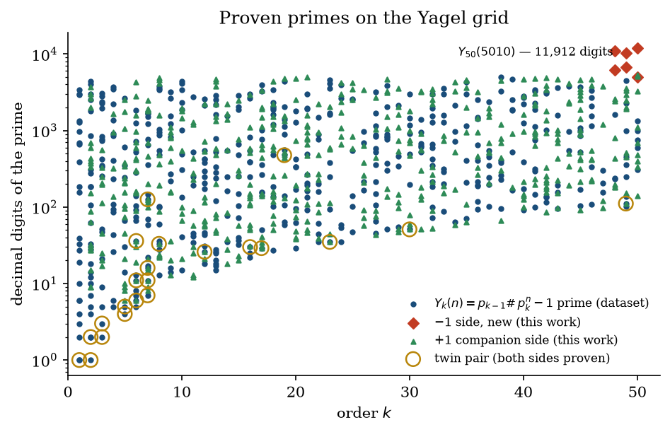
Statistics and computation (§4–5). Over the census domain of the original study ($k\le 50$, every exponent to 5000 digits; 482 minus-face primes, each proven) the sieve-adjusted prime-counting model fits the counts without free parameters, in aggregate and row by row; the Mersenne edge alone needs Wagstaff's additional divisor-class enrichment; prime exponents give the interior no measurable advantage; and cells prime on both faces occur at roughly the Hardy–Littlewood-adjusted rate. These are first-order model diagnostics over one fixed domain, not established laws. The same domain on the $+1$ face (§4.5) holds 484 primes over $k\in [2,50]$, and 22 cells are proven prime on both faces (§4.4). Running the same machinery forward (§5) yields primes far outside the domain — among the first, $Y_{50}(5010)$ of $\mathrm{11,912}$ digits, whose exponent $5010=2\cdot 3\cdot 5\cdot 167$ is emphatically composite.

Throughout, we are explicit about what the family does not offer (§6): the test, like Lucas–Lehmer, is $\tilde{O}(B^2)$ per candidate, and Mersenne retains its divisor-class enrichment and a smaller constant in its $\mathrm{\Theta }(B)$ reduction (Proposition 4 gives the interior the same linear-time reduction, with the bit-length of the primorial as the constant). The family's genuine assets are that every prime in it is provable by construction, that no cell is algebraically dead, and that the whole family is indexed by two parameters with no free choices.

2. Structure of the grid

2.1 The maximal small-prime sieve

Proposition 1. For every prime $q\le p_k$, $Y_k(n)\equiv -1(\mathrm{mod}q)$. In particular $gcd(Y_k(n),p_k\mathrm{\#})=1$: no prime up to the base divides any member of row $k$.

Proof. If $q<p_k$ then $q\mid p_{k-1}\mathrm{\#}$, and if $q=p_k$ then $q\mid p_k^n$; in both cases $q\mid Y_k(n)+1$. $◻$

The coefficient $h=p_{k-1}\mathrm{\#}$ is the smallest positive coefficient with $h{p}_k^n\pm 1\equiv \pm 1(\mathrm{mod}q)$ for every prime $q<p_k$: since $p_k$ is invertible modulo each such $q$, every one must divide the coefficient. Their product is necessary and sufficient; larger multiples also work.

This is the strongest clean congruence sieve available for the base: an integer $\equiv -1$ modulo every prime up to $p_k$. Quantitatively, coprimality to the first $k$ primes multiplies the prime density of a random integer of the same size by Mertens' factor

$$\begin{array}{}\text{(2)}& S_k=\prod _{q\le p_k}\frac{q}{q-1}\sim e^{\gamma }\ln p_k,\end{array}$$

which is the precise form of the intuition that the construction "amplifies" prime density (explicit estimates for (2) in Rosser–Schoenfeld [11]); §4 tests it against the data.

2.2 Every cell is live: no algebraic exponent filter

The Mersenne row loses all composite exponents to the identity $2^d-1\mid 2^n-1(d\mid n)$. The interior loses nothing:

Lemma 2. For $k\ge 2$, the polynomial $h{x}^n-1$ with $h=p_{k-1}\mathrm{\#}$ is irreducible over $\mathbb{Q}$ for every $n\ge 1$.

Proof. Up to a nonzero scalar, the reciprocal polynomial is $x^n-h$. Any prime dividing the squarefree integer $h>1$ divides its constant term but not its square and does not divide the leading coefficient. Eisenstein proves irreducibility. The same proof works for $x^n+h$, hence for the plus face. This says nothing about numerical coverings or infinitude of prime values. $◻$

So no polynomial identity in $p_k$ can divide $Y_k(n)$ for composite $n$: every exponent is a live candidate. The mechanism behind Mersenne's prime-exponent rule is exclusive to $h=1$. One can see the same fact locally: a prime $q>p_k$ divides $Y_k(n)$ exactly when

$$\begin{array}{}\text{(3)}& n\equiv t_q(\mathrm{mod}{\mathrm{ord}}_q(p_k)),t_q={\mathrm{dlog}}_{p_k}(h^{-1}modq),\end{array}$$

a shifted arithmetic progression in $n$. For $h=1$ all shifts vanish and divisibility aligns with the divisor lattice of $n$; for $h>1$ the shifts $t_q$ decouple divisibility from the multiplicative structure of $n$ entirely. §4.3 confirms statistically that prime exponents indeed confer no advantage — and three of the records in §5 have composite exponents.

Two honest caveats. Lemma 2 rules out polynomial identities, not covering systems: a hypothetical far row could still be Sierpiński–Riesel-style barren by a finite set of primes covering all residues (3). Two facts constrain that possibility.

Lemma 2′. For $k\ge 2$ and either face $h{p}_k^n\mp 1$, no prime kills all $n$ (period 1) or all $n$ of one parity (period 2). Every covering prime has ${\mathrm{ord}}_q(p_k)\ge 3$ and $q\ge p_{k+1}$.

Proof. A covering prime has $q\nmid h$, so $q>p_{k-1}$. Period 1 means $q\mid p_k-1$; but $p_k-1$ has no prime factor in $(p_{k-1},p_k]$. Period 2 means $q\mid p_k+1$ with $q$ odd, so $q\le (p_k+1)/2\le p_{k-1}$ by Bertrand's postulate, whence $q\mid h$ and $h{p}_k^n\mp 1\equiv \mp 1(\mathrm{mod}q)$. $◻$

In particular the "trivial" Riesel exclusion $gcd(c-1,b-1)>1$ of generic $c{b}^n-1$ searches never occurs on the grid. Computationally, no row $2\le k\le 1000$ is covered by the primes up to ${10}^5$ on either face (every row keeps survivors among $n\le 3000$, at the Mertens rate), and the largest covering density $\sum 1/{\mathrm{ord}}_q(p_k)$ achievable from primes of order $\le 12$ is $0.70$ (row 3), against the $1$ a covering needs; see §6. And Aurifeuillian-type numeric factorizations require cyclotomic values, which (1) does not produce.

2.3 Both neighbors factored

The central object of cell $(k,n)$ is $M=p_{k-1}\mathrm{\#}\cdot p_k^n$, with complete factorization known by construction. Its two neighbors are

$$M-1=Y_k(n)(\text{"}-1\text{ face"}),M+1=Y_k^{+}(n)(\text{"}+1\text{ face"}),$$

and for both, the adjacent number is fully factored: $N+1=M$ for the $-1$ face, $N-1=M$ for the $+1$ face. Consequently the classical $N+1$ (Brillhart–Lehmer–Selfridge / Morrison [1, 3]) and $N-1$ (Pocklington [4]; in single-exponentiation form, Grau–Oller-Marcén–Sadornil [17]) theories give every prime in either face a deterministic certificate at Lucas-chain cost — and when both faces are prime at the same cell they form a twin pair in which each member certifies cheaply (§4.4). This "always provable" property is what generic members of the $c{b}^n\pm 1$ genus lack unless $c$ happens to factor.

3. A Lucas–Lehmer-type test for every row

Throughout this section $N=Y_k(n)=h{p}^n-1$ with $h=p_{k-1}\mathrm{\#}$, $p=p_k$, and Lucas sequences $U_m,V_m$ have parameters $(P,Q)$ with $Q=1$, $D=P^2-4$, i.e. $V_0=2$, $V_1=P$, $V_{m+1}=P{V}_m-V_{m-1}$. Two classical facts (work in ${\mathbb{F}}_{r^2}$ for a prime $r\nmid 2D$, with $\omega =\alpha /\overline{\alpha }$ for the roots $\alpha ,\overline{\alpha }$ of $x^2-Px+1$):

1. $V_m={\alpha }^m+{\alpha }^{-m}$, so $V_m=2$ iff ${\alpha }^m=1$ and $V_m=-2$ iff ${\alpha }^m=-1$: multiply by ${\alpha }^m$ and use that a field has no nonzero nilpotents. Meanwhile $U_m=0$ iff ${\omega }^m=1$ with $\omega ={\alpha }^2$, allowing either V sign.
2. ${\mathrm{ord}}_r(\alpha )$ divides $r-\left(\frac{D}{r}\right)$: Frobenius fixes the roots in the split case and interchanges them otherwise.

Because $Q=1$, the $V$-sequence is closed under composition of indices: $V_{cm}(P)=V_c(V_m(P))$, where $V_c(x)$ is a monic degree-$c$ polynomial — the Chebyshev polynomial up to scaling, $V_c(2\cos \theta )=2\cos (c\theta )$ — evaluated modulo $N$ by a two-term "ladder" in $2\lceil {\log }_{2}c\rceil$ modular multiplications, with no $U$-values needed.

Theorem 3 (one-ladder test). Let $h,n$ be positive integers, $N=h{p}^n-1>1$, $p$ an odd prime, $p\nmid h$, and $p^n\ge h+2$. Suppose $P\ge 3$ satisfies $gcd(2D,N)=1$ and $\left(\frac{D}{N}\right)=-1$. Define

$$s_0=V_h(P)modN,s_{i+1}=V_p(s_i)modN(0\le i<n),$$

so that $s_i=V_{h{p}^i}(P)modN$ and $s_n=V_{N+1}(P)modN$. If

$$\text{(i)}{s}_n\equiv 2(\mathrm{mod}N)\text{and}\text{(ii)}gcd(s_{n-1}-2,N)=1,$$

then $N$ is prime. Conversely, prime $N$ satisfies (i) for every admissible trace, and a successful seed exists. A particular admissible seed may fail (ii).

Proof. For each prime $r\mid N$, (i) gives ${\alpha }^{N+1}=1$ and (ii) gives ${\alpha }^{(N+1)/p}\ne 1$. Thus the order divides $h{p}^n$ but not $h{p}^{n-1}$, so its p-adic valuation is n because $p\nmid h$. Consequently $p^n\mid r-(D|r)$ and $r\ge p^n-1$. If N were composite, its smallest prime divisor would be at most $\sqrt{N}$, including for repeated prime factors. But $(p^n-1{)}^2-N=p^n(p^n-h-2)+2>0$, a contradiction. The Jacobi condition is needed for prime-case necessity, not sufficiency.

For prime N the norm-one group has order M=N+1 and is cyclic. Exclude ±1; inversion pairs its remaining M−2 elements into admissible traces. The p-th power subgroup contains M/p elements including ±1 (p odd), leaving M/p−2 bad elements. Uniform admissible trace residues therefore succeed with $(N+1)(1-1/p)/(N-1)$, not exactly $1-1/p$. For N=17,p=3, six of eight admissible traces succeed. Sequential seeds have no expectation from this uniform law. $◻$

Parity also gives $2p^n\mid r\pm 1$, so $(2p^n-1{)}^2>N$ is a sharper sufficient bound. Production retains the conservative threshold; no new priority is claimed.

Remarks.

1. Classical edge. For N=2^n−1, n=1 gives 1 and n=2 gives 3. Composite n>1 factors N. For prime n≥3 the classical Lucas–Lehmer theorem starts at 4, iterates x²−2 exactly n−2 times and tests for zero modulo N. Arbitrary Jacobi-admissible seeds do not supply an unconditional iff test. The minus-two V condition is a sufficient order certificate; its converse needs the appropriate seed theorem, separately from the odd-p argument.

1. Certificates and retries. Under the theorem's hypotheses, a failure of (i) witnesses compositeness, a proper gcd exposes a factor, and gcd=N is inconclusive. Sequential seed retries have no proved expectation here.

1. Below the threshold. The regime $p^n\ge h+2$ — equivalently $n\ge n_0(k)\approx \ln p_{k-1}\mathrm{\#}/\ln p_k\sim p_{k-1}/\ln p_k$ by the prime number theorem — covers all but an initial segment of each row ($n_0(50)=38$; a $Y_{50}$ candidate at $n_0$ has 179 digits). Below it the same machinery applies with more factored primes of $N+1$ carried until the certified part exceeds $\sqrt{N}$ (Brillhart–Lehmer–Selfridge [1]); at most $k$ short ladders.

1. Cost. The ladder spends $2\lceil {\log }_{2}p\rceil$ multiplications per step and $n$ steps: about $2{\log }_{2}N$ multiplications total, versus $\approx 0.7{\log }_{2}N$ squaring-equivalents for one Fermat test — a proof for roughly the price of three PRP tests, at the same $\tilde{O}(B^2)$ bit complexity as Lucas–Lehmer. Mersenne's $\mathrm{\Theta }(B)$ modular reduction is inherited as well, in radix $p$ (Proposition 4 below); its constant is the bit-length of $h$.

1. Empirical validation. An implementation re-proved all 476 dataset primes in the one-ladder regime and rejected 100 composite controls with zero disagreements; seed retries were observed; this does not verify a random-seed runtime law. At scale, the ladder proved the $\mathrm{11,912}$-digit prime of §5 in 17.7 s (single seed, $P=4$) on commodity hardware — faster in practice than the equivalent $U$-sequence BLS routine (55.6 s).

1. Gcd-free form (Theorem 3′). Let ${\mathrm{\Psi }}_p$ be the minimal polynomial of $2\cos (2\pi /p)$, ${\mathrm{\Psi }}_p(x)=\prod _{j=1}^{(p-1)/2}(x-2\cos (2\pi j/p))=1+V_1(x)+\cdots +V_{(p-1)/2}(x)$ (degree $(p-1)/2$, integer coefficients; ${\mathrm{\Psi }}_3=x+1$, ${\mathrm{\Psi }}_5=x^2+x-1$), so that $V_p(x)-2=(x-2){\mathrm{\Psi }}_p(x{)}^2$ and ${\mathrm{\Psi }}_p(2)=p$. Under the hypotheses of Theorem 3, $N$ is prime iff ${\mathrm{\Psi }}_p(s_{n-1})\equiv 0(\mathrm{mod}N)$ for any seed that is not a $p$-th power: condition (i) is then automatic, a seed that is a $p$-th power shows itself as $s_{n-1}\equiv 2$ (and ${\mathrm{\Psi }}_p(2)=p\not\equiv 0$), and every other outcome is an exact compositeness witness. The proof is that of Theorem 3 with "${\alpha }^{(N+1)/p}$ is a primitive $p$-th root of unity modulo every prime factor $r$" read off from ${\mathrm{\Psi }}_p(s_{n-1})\equiv 0(\mathrm{mod}r)$. This is the shape of Lucas–Lehmer: ${\mathrm{\Psi }}_2(x)=x+2$ gives "$s_{n-1}\equiv -2$", and on row $k=2$ ($p=3$) the test reads iterate $x\mapsto x^3-3x$ from $P^2-2$ and demand the penultimate value be $-1$. Moreover $P=4$ is admissible on every cell with $k\ge 2$, since $N\equiv 1(\mathrm{mod}4)$ and $3\mid N+1$ give $(\frac{12}{N})=(\frac{N}{3})=-1$. Validated with zero disagreements on every cell with $N<2^{62}$ for $k\le 10$, on all dataset primes to 1500 digits, and on row 2 to $n=2000$.

Prior art. Explicit Lucas–Lehmer-type criteria for numbers $K{p}^n\pm 1$ have a long history that Revision 2.0 failed to cite: Williams [12] for $2A\cdot 3^n-1$ (1972), Bosma [13] for $h\cdot 2^k\pm 1$, Berrizbeitia–Berry [14, 15] for $A\cdot 3^n\pm 1$ and $A\cdot 5^n\pm 1$ via cubic and biquadratic reciprocity (explicit seeds), Stein–Williams [16] for $(p-1)p^n-1$, Grau–Oller-Marcén–Sadornil [17] for $K{p}^n+1$ with a single exponentiation (the $+1$ face) and [20] for $4K{p}^n-1$, Deng–Huang [18] for $h\cdot 2^n\pm 1$, and, most recently and most generally, Jakhar–Ram [19] (April 2026) for $K{p}^{\ell }-1$ with $K<p^{\ell }$: their criterion, ${\mathrm{\Phi }}_p(w^{K{p}^{\ell -1}})\equiv 0(\mathrm{mod}N)$ for $w$ in the unitary group $a^2-D{b}^2\equiv 1$, is Remark 6 in trace-free form. Theorem 3 is therefore a specialization, not a new test; it was derived for Revision 2.0 (July 2026) from the Brillhart–Lehmer–Selfridge theory [1] without knowledge of [19], which has priority for the general $-1$ form (the family itself, and the census, date from Revision 1.0, October 2024). What is specific to the grid is that the hypotheses (known adjacent factorization) hold by construction, while the one-ladder size bound holds only in its stated regime, the $V$-only Chebyshev-ladder presentation in which Lucas–Lehmer is the first row, the universal seed, and the campaigns of §5. Only the deterministic choice of seed for general $p$ (the analogue of [14, 15, 18] beyond $p=5$) remains open (§6).

3.1 Modular reduction in radix $p_k$

Mersenne's remaining arithmetic advantage was, until now, the shift-and-add reduction modulo $2^p-1$. It transfers.

Proposition 4 (fold at $N+1$). Let $N=h{p}^n-1$. For $X\ge 0$ write $X=A(N+1)+B$ with $0\le B\le N$. Then

$$X\equiv A+B(\mathrm{mod}N),\text{and}A+B\le 2N-1\text{ whenever }X<N^2.$$

In radix $p$, since $N+1=h{p}^n$, the pair $(A,B)$ is obtained by a shift of $n$ digits followed by one short division by the constant $h$; the reduction of a product therefore costs $\mathrm{\Theta }(B\cdot \log h)$ bit operations — linear in $B$ for a fixed row, as for Mersenne, which is the case $h=1$, $p=2$ (shift and add).

Proof. $N+1\equiv 1$, so $X\equiv A+B$. If $X<N^2$ then $A\le X/(N+1)<N^2/(N+1)<N$, so $A\le N-1$ and $A+B\le 2N-1$: one conditional subtraction finishes. In radix $p$, $\lfloor X/p^n\rfloor$ is a digit shift and $A=\lfloor \lfloor X/p^n\rfloor /h\rfloor$ a division of a $B$-bit number by a $\log h$-bit constant (schoolbook short division, or one product by a precomputed reciprocal of $h$), while $B=X-A(N+1)$ costs one more such product. $◻$

Remark (Montgomery form). Equivalently, with radix $R=p^n$ one has $R^{-1}\equiv h(\mathrm{mod}N)$ because $hR=N+1$, so Montgomery reduction is $\mathrm{REDC}(T)=T_{\mathrm{hi}}+h{T}_{\mathrm{lo}}\equiv Th$ — a multiplication by $h$ instead of a division. Montgomery's single-fold bound needs $T<NR\approx N^2/h$, so for a product of two residues the output can reach $(h+1)N$; a second fold at $N+1$ of its top $\lceil {\log }_p{h}^2\rceil$ digits (an $O({\log }^{2}h)$ division) brings it below $N+h+2$. Either way, one short operation with the primorial per modular multiplication.

The objection recorded in Revision 2.0 — that folding requires the dense constant $h^{-1}modN$ — was a representation artifact: folding at $N+1$ (or in Montgomery form) uses $h$ itself, exactly as Lucas–Lehmer–Riesel implementations do for $h\cdot 2^n-1$. Relative to the multiplication it reduces, the overhead is $\log h/B\approx n_0(k)/n$, the same threshold that governs the one-ladder regime: deep in that regime the interior is Mersenne-like in constants as well. A radix-$p$ limb implementation of the complete test, using digit shifts and short operations by $h$ only, agrees with the generic implementation on every cell tried. Existing production code (gwnum) reaches this speed for $h<2^{51}$, i.e. rows $k\le 14$; beyond that a large-coefficient weighted transform is an engineering task, not a mathematical one.

4. Statistics of the grid

The domain of this section. Everything in §4 is computed over one fixed domain, the census domain of the original study (Revision 1.0, 2024): orders $k\le 50$ and every exponent $n$ with $Y_k(n)<{10}^{5000}$, the rows running from $(1,16609)$ to $(50,2081)$. The domain is fixed because it is the original study's; it serves this section as a benchmark for the model comparisons, and it is not a description of how far the project's computations now extend, which the published index records (§5.2). The plus face is taken over the same cells with $k\in [2,50]$ (§4.5); its row $k=1$ is the Fermat form and is treated by algebra.

The domain is completely decided. On the minus face it holds 482 primes. Each is proven: it carries a stored certificate that replays against its own coordinates under the criteria of §3, or trial division below $2^{20}$. $Y_1(1)=1$ is neither prime nor composite. Every other cell is composite, and each carries a compositeness witness for the integer its coordinates name, computed from those coordinates: a proper divisor, or failing that a strong probable-prime test to base 2 that the integer fails for $k\ge 2$ — on the Mersenne row, the algebraic factor $2^d-1$ of a composite exponent or a failed Lucas–Lehmer test instead, since base 2 cannot witness there (every $2^q-1$ with $q$ prime passes it). The plus face is decided the same way, with the algebraic factors of $2^n+1$ and Pépin's test on its first row. A witness decides its integer outright, so these composite verdicts are not a weaker grade of evidence than the prime certificates, and none of them is inferred from a cell's absence from the prime list. They also do not rest on the classifications of the 2024 sweep, of which a 2026 re-test found six wrong (errata, Revision 2.1): every composite cell was witnessed afresh from its coordinates, and the published index declares the verdict of every cell of the domain on both faces.

Except where stated, counts are taken over the window 100–5,000 digits, wide enough that boundary effects and the heuristic's small-$N$ breakdown are immaterial. Later searches reported in §5 are not part of this domain: they target large exponents in chosen rows and are not census samples, so they are never pooled with the counts below.

4.1 A first-order model for the census counts

The correct null model for a family satisfying Proposition 1 is not the bare prime number theorem but PNT conditioned on the built-in sieve: a candidate of size $Y$ is prime with probability $\approx S_k/\ln Y$ with $S_k$ from (2) — computed exactly, not asymptotically. Expected counts per row are then $E_k=\sum _n{S}_k/\ln Y_k(n)$ over the window.

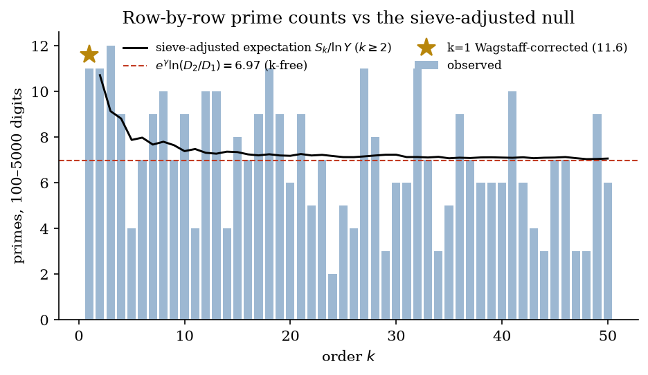
Result. Over the census domain restricted to $k\in [2,50]$ and the 100–5,000-digit window: $344$ primes observed against $361.8$ expected, a Poisson $z$ of $-0.94$, with $|z|<2$ in every individual row (Fig. 2). The census counts are consistent with the first-order sieve heuristic over this domain. The "higher than expected density" reported in Revision 1.0 is accounted for by the Mertens factor (2), with nothing left over. This is a model diagnostic over one fixed domain, not evidence that the counts follow a Poisson law.

A pleasant closed form follows from $E_k$: over a digit window $[D_1,D_2]$,

$$\begin{array}{}\text{(4)}& E_k\approx \frac{S_k}{\ln p_k}\ln \frac{D_2}{D_1}\approx e^{\gamma }\ln \frac{D_2}{D_1},\end{array}$$

independent of $k$ — the Mertens boost cancels the thinning from the larger base. For the window of Fig. 2 this predicts $e^{\gamma }\ln 50=6.97$ primes per row, and the observed counts do cluster around 7 across all fifty rows. The scatter is summarized against a Poisson reference, which is a descriptive choice here: the exponent sieves of the next paragraph are dependent, so that reference is not a calibrated uncertainty model.

Dependent exponent sieves. For each explicit prime q>p, divisibility excludes at most one phase modulo ord_q(p). These periods share factors. For h=2,p=3,Q={5,7}, minus excludes 1 mod 4 and 4 mod 6: seven of twelve exponents survive. Plus excludes 3 mod 4 and 1 mod 6: eight survive. The marginal-independence product is 5/8 for both and is therefore not the joint density. Dividing exact survivals by (1−1/5)(1−1/7) gives finite corrections 245/288 and 35/36, versus the baseline 175/192.

Exact rational period counts, and explicit finite-window counts with their phase residues, are computed directly rather than estimated from a product; the earlier numeric product is retained only as an explicitly named marginal-independence baseline. Divisibility by $q$ at $N=q$ does not establish compositeness. Neither finite correction establishes an infinite prime-count constant, and the refined fits and $z$-scores of Revision 2.1, which rested on the product, are withdrawn. The first-order fits above remain descriptive statements about this domain.

4.2 The Mersenne edge is different in kind — measurably

Row $k=1$ under the naive restricted null (prime exponents only, probability $2/\ln M_q$) predicts only $1.5$ primes in the window; $11$ are observed. The discrepancy is Wagstaff's [6]: divisors of $2^q-1$ lie in the classes $\pm 1mod8$ and $1mod2q$, enriching surviving candidates by a factor $\sim e^{\gamma }\log (aq)/\log 2$. The corrected prediction is $11.6$ — against 11 observed. The interior rows, by contrast, fit without any such correction: divisors obey the shifted-progression law (3), whose joint correlations require further analysis. The grid thus cleanly separates the two Mersenne gifts: the edge keeps its divisor-class enrichment; the interior trades it for Lemma 2's universality of live cells.

4.3 Prime exponents: no advantage visible in this domain

Lemma 2 says no exponent is disqualified algebraically. Whether prime exponents are nonetheless favored is a separate, empirical question. Split every interior cell of the census domain ($k\ge 2$, $n\ge 2$) by the primality of its exponent and normalize each group by its summed sieve-adjusted expectation:

The expectation-normalized rate ratio (prime exponents : composite exponents) is $1.079$. Carrying that through the Poisson reference of §4.1 at nominal 95% gives $[0.870,1.340]$ — but §4.1 has just said that reference is not a calibrated uncertainty model here, because the exponent sieves are dependent, so this interval is a conditional calculation under a model that is not validated and no coverage claim attaches to it. Read descriptively, the two groups sit close to a common expectation and the ratio is within the range the arithmetic of a domain this size would put around 1. That is the whole of what the table shows: it neither exhibits an exponent effect nor establishes that there is none. The large primes of §5 illustrate the point concretely: $Y_{50}(5010)$ has exponent $2\cdot 3\cdot 5\cdot 167$ and $Y_{49}(4319)$ has $7\cdot 617$ — primes of many thousands of digits in cells that have no counterpart on the Mersenne row, where such exponents are excluded outright.

4.4 Cells prime on both faces

When both faces of a cell are prime, $(M-1,M+1)$ is a twin-prime pair in which each member has a completely factored neighbor — so both are proven at Lucas-chain cost, which generic twin constructions cannot offer. Over the census domain, 22 cells are prime on both faces, at

$$(k,n)\in \{(1,2),(2,1),(2,2),(3,1),(3,2),(5,1),(5,2),(6,2),(7,2),(6,6),(7,5),(7,9),(12,9),(17,5),(16,7),(8,21),(23,2),(6,29),(30,3),(49,10),(7,98),(19,248)\},$$

the largest being $(Y_{19}(248),Y_{19}^{+}(248))=p_{18}\mathrm{\#}\cdot {67}^{248}\mp 1$, of 476 digits each. Twenty-one of the 22 lie at $k\ge 2$; the twenty-second is $(1,2)$, which the next paragraphs treat separately.

How many a heuristic expects, and where the heuristic stops. Both faces of a cell avoid every prime $q\le p_k$ by construction: $M\equiv 0$, so $M\mp 1\equiv \mp 1$. For $q>p_k$ the model assumes that $M$ is uniform over the residues mod $q$, which kills the pair with probability $2/q$ — two forbidden residues rather than one. That assumption is the model's weakest part and is not satisfied here: as $n$ runs, $M=p_{k-1}\mathrm{\#}{p}_k^n$ moves through a multiplicative orbit mod $q$ rather than over all residues, the same dependence §4.1 documents for the single-face sieve. Against the local density of a random pair, $(1-1/q{)}^2$, the assumption gives a cell probability $T_k/(\ln Y_k(n){)}^2$ with

$$\begin{array}{}\text{(6)}& T_k=\prod _{q\le p_k}(1-\frac{1}{q}{)}^{-2}\prod _{q>p_k}(1-\frac{1}{(q-1{)}^2})=S_k^2{C}_2/\prod _{3\le q\le p_k}(1-\frac{1}{(q-1{)}^2}),\end{array}$$

$S_k$ as in (2), $C_2=0.6601618\dots$ the twin-prime constant [10], and the tail taken over $q$ strictly greater than $p_k$ — so $T_2=12C_2$ and $T_3=20C_2$.

Summed over $k\in [2,50]$ and every exponent of the domain, (6) comes to 24.31, against the 21 twin cells the census holds at $k\ge 2$. That figure is printed as a diagnostic of the model and not as an expectation: two of its terms, at $(2,1)$ and $(3,1)$, exceed 1, and a "probability" above 1 is the heuristic stating that it does not apply. Those two sit inside the 87% of the sum contributed by cells below 100 digits, where $\ln Y$ is small enough that the density is meaningless whether or not the individual term crosses 1.

Over the 100–5,000-digit window in which §4.1 operates, (6) gives 3.07 and the census contains 3 — at $(7,98)$, $(49,10)$ and $(19,248)$. Three cells discriminate between nothing; the agreement is recorded, not leaned on. With the uniformity assumption unmet, no interval and no significance statement attaches to either figure. Everything the sum needs is stated here — the domain, the constant, the tail's range, the exclusion of row 1, the logarithm taken at $Y=M-1$ — so it is a finite sum of 146,685 terms, recomputable from that specification alone.

Row $k=1$ is outside (6), and not for convenience: $M=2^n$, so $M-1$ requires $n$ prime and $M+1$ requires $n$ a power of two. Only $n=2$ meets both, and it is prime on both faces — the pair $(3,5)$. Algebra fixes row 1 at exactly one twin cell, which is what the census finds, and the generic model cannot be evaluated there to compare: its $n=1$ term divides by $\ln Y_1(1)=\ln 1=0$. Searches outside the census domain have since found further such cells at larger $k$; they are catalogued separately and are not part of the count above.

4.5 The plus face

The second kind $Y_k^{+}(n)=p_{k-1}\mathrm{\#}{p}_k^n+1$ is not a Mersenne generalization — it lives in the $c{b}^n+1$ branch of the genus — but it is the same grid seen from the other face, and the structure transfers wholesale: it satisfies the same Proposition 1 (with $+1$ in place of $-1$); Lemma 2 holds verbatim ($x^n+h$ is irreducible for all $n$ when $h$ is squarefree $>1$, by the same Eisenstein argument applied to the reciprocal polynomial), so its interior has no dead cells either; and it is proven by Pocklington's $N-1$ test instead of the Lucas $N+1$ test. Its classical edges mirror the first kind's: the $n=1$ column is the Euclid numbers $p_k\mathrm{\#}+1$ (Caldwell–Gallot [8]), and the $k=1$ row, $2^n+1$, is the one line of the whole two-faced grid that is algebraically gated — $a^d+1\mid a^n+1$ for $n/d$ odd, so only $n=2^m$ (the Fermat numbers) survive. Both faces thus have exactly one exceptional edge each ($h=1$) and fully live interiors.

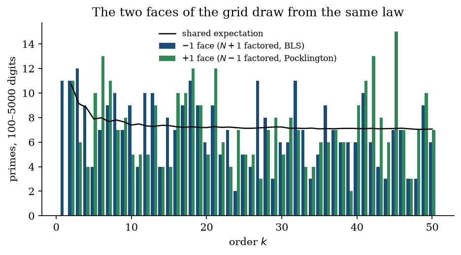
The sieve-adjusted model of §4.1 draws no distinction between the two faces, and that prediction was registered before the plus face was swept. Over the same grid ($k\in [2,50]$, all $n$ to 5,000 digits) the plus face holds 484 proven primes, and every other cell is witnessed composite as described at the head of §4. In the 100–5,000-digit window the plus face has 357 primes against a predicted 361.8 ($z=-0.25$, counting the boundary cell $Y_{21}^{+}(2669)$ at exactly 5,000 digits, which Revision 2.0 omitted), and the minus face 344 against the same expectation ($z=-0.94$). Fig. 3 shows the two counts row by row. This is agreement between two observed count sequences and one first-order expectation over one domain; it is not evidence that the faces obey an identical joint law.

The sweep also doubled the family's inventory of proven primes in a single computation, which is §2.3 in practice: every candidate the sweep turned up was carried through to a certificate in the same pass, so the sweep's output is a list of theorems rather than a list of leads. The largest members of the plus-face census are $Y_{21}^{+}(2669)=p_{20}\mathrm{\#}\cdot {73}^{2669}+1$ (5,000 digits), $Y_{42}^{+}(2139)$ (4,900) and $Y_8^{+}(3806)$ (4,873).

4.6 Limiting density: an open question

Mertens' theorem gives $S_k/\ln p_k\to e^{\gamma }$ for the sieve-only factor. It does not give a limit for a dependent row correction, nor a prime-count asymptotic along exponential sequences, and the two are different questions. The claims $C_k\to 1$ and $A_k\to e^{\gamma }$ made in Revision 2.1 are withdrawn: they were read off per-row products of marginal survival factors, and §4.1 shows those factors are dependent, so the products are a baseline computed under an assumption that does not hold rather than estimates of anything. No justified limiting constant is presently available.

Two approaches do not settle this. Simulating a generic coefficient changes the probability space, so it answers a different question. Comparing a heuristic with the same counts that suggested it cannot calibrate its uncertainty. A prospective test would need a census block reserved in advance and left untouched; no such holdout is claimed here.

5. Searching at scale

The properties of §2–3 assemble into a pipeline in which discovery and proof are the same pass:

1. Sieve. For fixed $k$, mark exponents $n$ killed by primes $p_k<q\le L$ via the rolling recurrence $r\leftarrow r{p}_{k}modq$ against the target residues of (3) — one pass per $q$, both faces simultaneously if desired.
2. PRP. Survivors take one Fermat test base 2 (the theoretical minimum: one modular exponentiation), then a BPSW check.
3. Certificate. A survivor of step 2 is a candidate, not yet a prime. Theorem 3 (or its Pocklington mirror on the $+1$ face) is then attempted against it, at $\sim 3\times$ the cost of step 2; in the one-ladder regime that is a single ladder with a seed that must succeed, and below the regime it is the multi-factor argument of Remark 3. A value enters the record only when the applicable criterion returns a certificate, and that certificate is stored and replayed. What the grid buys is that step 3 is always available and cheap, never that step 2 already settled the question.

A cost identity parallels (4): at sieve depth $L$, surviving candidates per digit window number $\approx dD\ln 10/\ln L$ and expected primes $\approx e^{\gamma }dD/D$ — both $k$-free — so **tests-per-prime, $\approx D\ln 10/(e^{\gamma }\ln L)$, is the same on every interior row.** There is no privileged row to search; larger $k$ merely takes fewer, larger exponent steps per digit. (The Mersenne edge is privileged, by precisely its Wagstaff factor of §4.2.)

5.1 The first forward campaigns (June–July 2026)

These are campaign results, not census results. The searches below target chosen rows and large exponents; they sample no domain exhaustively and are never pooled with the counts of §4. Each value listed was carried from candidate to certificate in the same pass, and is listed only because that certificate succeeded. The first forward campaigns ran in June–July 2026 on a commodity 8-core desktop with GMP arithmetic and produced:

The first prime in rows beyond $k=50$. For each new row we searched upward from $n=1$ until a prime appeared, and proved it. The result is the first prime found in that row; calling it the row's smallest prime exponent would require every smaller exponent to have been settled composite, which these searches sieved for but did not individually prove. This was done for every $k\in [51,100]$ and for milestone rows $k=150,200,300,500,750,1000$: fifty-six first-of-row primes, every one of them proven, from $Y_{51}(4)$ ($101$ digits) to

$$Y_{1000}(1098)=p_{999}\mathrm{\#}\cdot {7919}^{1098}-1(\mathrm{7,670}\text{ digits}),$$

the latter found after 856 Fermat tests ($\approx 14$ minutes on one core) and proven in 16 s by Theorem 3 — its exponent lies above the one-ladder threshold $n_0(1000)\approx 874$. The first prime of row $k=750$ ($n=548$, $\mathrm{4,490}$ digits) falls below its threshold and exercised the multi-factor certificate of Remark 3 (115 s). The same campaign on the $+1$ face opened all fifty-six rows as well and produced the largest prime of these campaigns — later searches have gone well past it: row 1000's $+1$ face resisted until $n=3918$ — $\mathrm{3,079}$ Fermat tests, under five hours on one core — yielding $Y_{1000}^{+}(3918)$ with $\mathrm{18,664}$ digits, proven by Pocklington in 24 s and confirmed by a 50-round Miller–Rabin control. These first exponents scatter roughly as the long-tailed geometric distribution implied by a per-cell success probability $\approx S_k/\ln Y$: most rows yield a prime within a few dozen exponents, while row 100, for instance, resists until $n=1279$ ($\mathrm{3,713}$ digits). A single big-integer gcd against the primorial of all primes to ${10}^5$ served as the entire trial-division stage for these searches — a convenience specific to a family born coprime to every small prime.

Proving times illustrate Remark 4: the $\mathrm{11,912}$-digit record took 31 s for the Fermat test, 17.7 s for the one-ladder certificate (seed $P=4$, first try), and 55.6 s for the equivalent $U$-based BLS routine; all three verdicts, plus a 50-round Miller–Rabin control, agree. Yields were compared with the predictions of (4), which were fixed before the searches ran: across the nine 5,000–7,000-digit row-faces searched, 5.4 expected and 5 found; in the 10,000–12,000-digit windows, 1.1 expected and 3 found; in the plus-face census of §4.5, 362 expected and 357 found; and in a 20,000–26,000-digit probe of row 50, 0.47 expected and none found. Four comparisons over four differently chosen windows are a sanity check on the order of magnitude of (4), not a test of it.

5.2 The catalogue and its releases

§4 is a census over one fixed domain and §5.1 is one pair of campaigns. Neither is the project's accumulated record, which grows with every search and is therefore not restated here. It is published as two versioned data releases, and a figure drawn from them should be cited with the version stamp the files carry.

The catalogue of proven primes (yagelnumbers.org/primes, machine-readable at yagelnumbers.org/data/primes.json) lists a value only when it carries a stored certificate that replays against its own coordinates. The criteria are the two of §3 and §4.5 — Lucas $N+1$ on the minus face, Pocklington $N-1$ on the plus face — with trial division below $2^{20}$. A certificate that names an integer other than the one its coordinates define is rejected, not reinterpreted. The method under which an older value was originally found is history, not the grounds on which it is published.

The index (yagelnumbers.org/data/index.json) records, for each row and face, the exponent ranges in which every cell is decided — each prime by its certificate, every other cell by a compositeness witness of the kinds described at the head of §4. Inside such a range a cell that is not a listed prime is composite because it was witnessed, not because it is absent from the list; outside every such range, and with no certificate of its own, a cell is unknown. The calculator at yagelnumbers.org/datasets answers from the same rule, and reports $Y_1(1)=1$ as neither prime nor composite.

What a count of primes is not. A total of proven primes is not a claim about the regions they were found in. Much of the catalogue comes from targeted searches over chosen rows and exponent windows, and a prime found at one exponent says nothing about its neighbors; coverage is what the index states, range by range, and nothing more.

6. What the grid is, and is not

It is not a complexity breakthrough, and its test is not new. Per candidate, Fermat, Miller–Rabin, Lucas–Lehmer, and Theorem 3 are all $\tilde{O}(B^2)$ with fast multiplication, and Theorem 3 is a specialization of the classical $K{p}^n\pm 1$ criteria [12–20]. Mersenne keeps Wagstaff's divisor-class enrichment of its candidates — (3) shows the interior's divisor classes average flat, up to the historical marginal-product baseline (now withdrawn as a joint model) — and a smaller constant in its linear-time reduction ($h=1$ against $\log h$ in Proposition 4).

It is the canonical two-parameter interpolation between the Mersenne and primorial families, with four universal gifts: a maximal built-in sieve (Proposition 1), polynomial irreducibility in the interior (Lemma 2) and no cheap coverings (Lemma 2′), a certificate for every prime ever found in it (Theorem 3 and its mirror) — the property that distinguishes it inside its genus, where certificates exist only when the coefficient happens to factor — and Mersenne's linear-time reduction in its own radix (Proposition 4). Its finite statistics motivate further study but establish neither a Poisson process nor limiting row constants. And the evidence has a boundary worth stating plainly: every prime reported here was proven, and its certificate re-checked, by this project's own implementations. Replay in a second system covers a sample of the catalogue, not all of it, and external recertification by an independent party has not been carried out. No proof archive or independent verifier is published.

Open problems.

1. Optimality of Proposition 4: can the product by $h$ be amortized so that the reduction is $\mathrm{\Theta }(B)$ with a constant independent of the row — or is $\mathrm{\Theta }(B\log h)$ the truth? And, practically, a weighted-transform implementation for $h\ge 2^{51}$ (rows $k\ge 15$), where current production code falls back to generic arithmetic.
2. Covering systems: Lemma 2′ excludes periods 1 and 2 and no row $k\le 1000$ is covered by the primes to ${10}^5$, but whether any row is barren remains open; a proof would need control of the prime factors of ${\mathrm{\Phi }}_d(p_k)$ above $p_k$.
3. Deterministic seeds: the $p$-th-power condition of Theorem 3 is resolved by reciprocity for $p=2,3,5$ [13–15, 18]; on the grid the coefficient is fully known modulo everything, so an explicit seed per row may be provable for all $p_k$.
4. The $k>50$ and $n=1$ frontiers: the primorial-prime column is classical [7, 8]. Beyond the census domain, the smallest prime exponent of a row is known only where the index (§5.2) records every smaller exponent as decided; the first primes found beyond $k=50$ (§5.1) are not claimed to be the smallest.
5. Twin records within the family: because both members are provable, the grid is a natural venue for large proven twins beyond the 476-digit pair of §4.4 — though at the twin top-twenty threshold of September 2026 (71,298 digits) the expected yield per million cells is below $0.1$.

Scientific errata

Corrections are recorded here rather than applied silently. The historical PDF of Revision 1.0 is preserved uncorrected; it is not the current edition.

Revision 2.1 (September 2026) — census errata. A BPSW re-test of every cell of the 2024 census found six values it had recorded as composite that are in fact prime: $Y_{19}(6)$ and $Y_{19}(7)$ (35 and 37 digits, so row 19 opens at $n=6$), $Y_{15}(2121)$, $Y_{15}(2345)$, $Y_{15}(2757)$ and $Y_{25}(2379)$ (3,563 to 4,762 digits). All six are now proven and are included in every count in §4. The other 162,776 cells the 2024 sweep had classified composite were re-tested and again came back composite. (That figure excludes $Y_1(1)=1$, which earlier revisions carried inside the composite total; it is neither prime nor composite.) Those classifications rest on the re-test, not on a stored certificate, and this erratum is itself the demonstration that a sweep's record can misstate a cell: six is the number of misstatements that were found, not a bound on how many there are. The consequence for §4 is arithmetic, not structural: the minus-face census total moved from 476 to 482 and row 19's first prime moved earlier.

Revision 2.2 (September 2026) — three errors in Revision 2.1.

1. A product of marginal survival factors was treated as a joint density. Exponent periods modulo different primes share factors, so the factors are dependent and their product is not the survival density. §4.1 now gives exact finite-sieve counts instead, and the refined fits and their $z$-scores that rested on the product are withdrawn.
2. The $V$-sequence argument used a root ratio in place of a root. Modulo 7 with $P=3$ one has $V_4=-2$ while ${\omega }^4={\alpha }^8=1$, so the ratio does not carry the order argument. §3 now works with $\alpha$ itself.
3. The exact seed-success fraction omitted the excluded traces. The corrected count is $(N+1)(1-1/p)/(N-1)$, not $1-1/p$; see the proof of Theorem 3.

Revision 2.3 (September 2026).

1. Figure 4 is withdrawn. It plotted per-row products of marginal survival factors as though they were estimates of prime-count constants. Following erratum 1 above, those products are a baseline computed under an independence assumption that does not hold, they have no established coverage, and no limiting constant is claimed for them. The figure is removed rather than relabelled; the open question it was meant to illustrate is stated plainly in §4.6 and its research source is retained with the project's records.
2. Historical counts are now reported with their domain. §4's statistics are a census result over $k\le 50$ to 5,000 digits; §5's records are the July 2026 campaign. Neither is the current project catalogue, which is larger and is published separately. Earlier revisions printed these numbers without always distinguishing them.
3. The plus-face census total is corrected from 470 to 484. The 2026 sweep recorded 470 primes. Fourteen further plus-face primes in the same domain, all of 1 to 5 decimal digits at $k\le 5$ and below the exponent at which the sweep began, were established afterwards by the twin companion scan and by bounded trial division. The statistical window of §4.5 (100–5,000 digits) contains none of them, so the fit reported there is unchanged.

Revision 2.4 (September 2026). Five places where Revision 2.3 claimed more than the evidence behind it. Each surfaced on checking the text against the published index and calculator.

1. The census domain's size was wrong, and the value 1 was counted as composite. The domain as defined — $k\le 50$, $Y_k(n)<{10}^{5000}$ — contains 163,294 minus-face cells, from $(1,16609)$ to $(50,2081)$. The figure 163,259 printed in earlier revisions is the 2024 sweep's stored extent, which falls 1 to 3 exponents short of the cap on some rows; the 35-cell tail was settled separately in 2026. Within the domain, $Y_1(1)=1$ is neither prime nor composite and had been carried inside the composite total; the composite count is 162,811, and for the 2024 sweep alone 162,776.
2. Reported coverage was described as a settled classification. The 482 minus-face primes and the 484 plus-face primes are proven. The classifications over the rest of the domain come from the sweeps that covered them — the Revision 2.1 erratum above is itself a case of six of them being wrong — and the published index declares a cell composite only where completion evidence exists, answering unknown elsewhere. §4 now says so, and no longer speaks of the census "settling" its domain. (Revision 2.5 corrects how §4 said it.)
3. Screening was described as proof. §5's pipeline said a survivor of the PRP stage is "immediately proven" by Theorem 3, and the abstract that searching and proving are the same act. A survivor is a candidate; the criterion is then attempted and may need a different seed, or the multi-factor form below the one-ladder threshold. Relatedly, the grid supplies the factored-neighbor hypothesis at every cell by construction, not every hypothesis of the criteria; the abstract and the site said the latter.
4. An uncalibrated interval was reported as a 95% interval. §4.1 states that the Poisson reference is not calibrated here because the exponent sieves are dependent. §4.3 nonetheless attached nominal 95% coverage to a rate-ratio interval and read it as detecting no effect. The interval is retained as a conditional calculation with no coverage claim, and the section no longer asserts an absence of effect.
5. Appendix A promised implementations that are not distributed. It said reference implementations accompany the data; the availability section, correctly, says the code is not published. Appendix A is a specification to reimplement from.

Revision 2.5 (September 2026). Three corrections, all of them to statements Revision 2.4 introduced or left standing.

1. An expected twin count that could not be reproduced from its own specification. §4.4 reported a sieve-adjusted Hardy–Littlewood expectation of $27.2$ pairs against 22 observed, and read the gap as indistinguishable from chance. The figure dates from a July 2026 working note whose summand, limits and treatment of row 1 were never published, and it cannot be recovered from the paper as written; the same note records that its model gave row 1 about 3.5 pairs, where algebra permits exactly one. The expectation is withdrawn and replaced by (6), a bounded sum over a stated domain with row 1 excluded on algebraic grounds and recomputable from the specification printed with it. It is numbered (6), not (5): (5) was the row-constant product withdrawn in Revision 2.2 and that number is not reused. The sum comes to 24.31 over the whole domain at $k\ge 2$ against 21 observed there — printed as a diagnostic, since two of its terms exceed 1 and 87% of it comes from cells below 100 digits — and to 3.07 against 3 observed in the 100–5,000-digit window. The uniform-residue assumption behind it is now stated where it is used. No inference from the comparison is offered.
2. Historical classifications were written as current composite declarations. Revision 2.4 said the remaining cells "are declared composite on probabilistic screening, which is not the same grade of evidence". That misplaces the uncertainty. A Fermat or Miller–Rabin test that produces a witness decides compositeness outright — the doubt is over execution, coverage and the association of a recorded verdict with a cell, not over the mathematics. The abstract and §4 now say that, exclude $Y_1(1)=1$ explicitly, and describe the 162,811 as cells outside the proven-prime list carrying the sweeps' classifications.
3. A sentence in §4.3 asserted more than the section could support. "Only a reference with calibrated coverage could do the latter" is false as stated: calibrated coverage would not by itself establish the absence of an effect. The sentence is removed; the limited conclusion before it stands.

One further change was an addition rather than a correction: §5.2 gave a dated summary of the current catalogue, which earlier revisions had left entirely to the website, so that the paper no longer reported June–July 2026 as though it were the present state. Revision 2.6 replaces that summary with a pointer to the versioned releases.

Revision 2.6 (September 2026). The paper no longer restates figures that change with the dataset, and three statements are brought up to date.

1. The census domain is completely decided. Revisions 2.4 and 2.5 described the census cells outside the prime lists as carrying the 2024 sweep's classifications, and said the index answered unknown where it could not vouch for them. Every cell of the domain on both faces, save $Y_1(1)=1$, has since been witnessed composite from its own coordinates or, for the primes, certified, and the index declares each verdict. §4 and the abstract now state the domain as a complete enumeration and name the kinds of witness; the six false composites of the Revision 2.1 erratum are the reason the verdicts were re-derived rather than carried over.
2. Current catalogue figures are withdrawn from the paper. Revision 2.5 added to §5.2 a dated summary of the catalogue — its totals, the largest primes and a verified-coverage share of 0.25%. The share was overtaken within days, and the totals change with every search. §5.2 now states how the catalogue and the index are built and what they declare, and the figures themselves are published only in the versioned data releases. The paper's remaining figures are results over the fixed census domain, the dated campaigns of §5.1, and model quantities recomputable from their stated specifications.
3. A campaign record was described as the minus face's largest prime. §1 called $Y_{50}(5010)$, of $\mathrm{11,912}$ digits, the largest prime of the minus face; it was the largest minus-face prime of the June–July 2026 campaigns, and larger minus-face primes were already catalogued. §1 now says so.

What the claims below establish

Data and code availability

What a reader can obtain today. The catalogue of proven primes is published at yagelnumbers.org/data/primes.json, giving for each prime its order, exponent, face, digit count and the criterion its proof used. The per-order primality index, which carries the settled exponent ranges behind the composite verdicts, is at yagelnumbers.org/data/index.json. Any individual value can be recomputed and looked up at yagelnumbers.org/datasets. Each file carries a version stamp. The catalogue and the index grow with every search, so this paper does not copy their totals; a figure taken from them should be cited with the version it was read from.

What is not published. The certificates themselves — the witness data for each proof — the compositeness witnesses, and the search, proving and analysis code are held with the project and are not distributed. A reader therefore cannot re-run a proof from published material alone, and the results here rest on this project's own implementations. Appendix A specifies the algorithms in enough detail to reimplement them independently, which is the only route to a reader-side check at present.

The paper (text and figures), the catalogue and the dataset are released under the Creative Commons Attribution 4.0 license (CC BY 4.0) — reuse freely with attribution.

Acknowledgments

This work was carried out with AI assistance throughout: in the computation, in the verification tooling, in drafting, and in review. Every numerical claim in this paper is backed by a script that recomputes it. The mathematical responsibility for the results, and for the corrections recorded in the errata, is the author's.

Appendix A. Algorithms

The pseudocode below is the general form of the implementations actually used (Python, arbitrary-precision via GMP). The implementations themselves are not distributed — see Data and code availability — so this appendix is a specification to reimplement from, not a pointer to code a reader can obtain. V(c, P, N) denotes the $V$-only Lucas ladder for $Q=1$: state $(V_j,V_{j+1})$ over the bits of $c$, with $V_{2j}=V_j^2-2$, $V_{2j+1}=V_j{V}_{j+1}-P$ — two multiplications per bit.

Algorithm 1 — one-ladder certificate for $N=h{p}^n-1$ (Theorem 3; $p$ odd, $p^n\ge h+2$).

function OneLadder(h, p, n):
    N <- h * p^n - 1
    for P in 3, 4, 5, ...:                      # seed search
        D <- P^2 - 4
        if gcd(D, N) is a proper divisor: return COMPOSITE
        if Jacobi(D, N) != -1: continue
        s <- V(h, P, N)                          # seed  V_h
        repeat n times:
            prev <- s
            s <- V(p, s, N)                      # V_m -> V_{p*m}
        if s != 2 (mod N):        return COMPOSITE          # exact
        g <- gcd(prev - 2, N)
        if g == 1:                return PRIME               # certificate
        if g < N:                 return COMPOSITE           # factor found
        # g == N: seed was a p-th power (inconclusive; no sequential probability claim) - next P

For $k=1$ ($p=2$, map $x\mapsto x^2-2$) replace the final two conditions by prev == -2 (mod N) — the Lucas–Lehmer(–Riesel) form. Below the one-ladder threshold, run the same ladder for each carried prime $q\mid N+1$ largest-first until the certified part exceeds $\sqrt{N}$ (Brillhart–Lehmer–Selfridge [1]).

Algorithm 2 — proven search over a row (§5; either face).

function HuntRow(k, n1, n2, sieve limit L, face e in {-1,+1}):
    h <- p_{k-1}# ; p <- p_k
    alive[n1..n2] <- true
    for each prime q in (p_k, L]:                # sieve: shifted APs (3)
        t <- -e * h^{-1} mod q                   # p^n = t (mod q) => q | h p^n + e
        r <- p^{n1} mod q
        for n = n1..n2:
            if r == t and h*p^n + e > L^2: alive[n] <- false
            r <- r * p mod q
    for n = n1..n2 where alive[n]:
        N <- h * p^n + e
        if 2^{N-1} != 1 (mod N): continue        # Fermat, base 2
        if not BPSW(N): continue                 # PRP confirmation
        prove: e = -1 -> Algorithm 1 (N+1 side)
               e = +1 -> Pocklington on N-1      # same ladder economics
        record proven prime (k, n, e)

Algorithm 3 — first prime of a row (§5): iterate $n=1,2,\dots$ with a single big-integer screen gcd(N, Q#) where Q# = product of all primes <= 10^5 in place of the sieve (deciding exactly when the gcd equals $N$ itself), then proceed as in Algorithm 2. The first $n$ whose value is proven prime is the one reported for that row.

References

[1] J. Brillhart, D. H. Lehmer, J. L. Selfridge, New primality criteria and factorizations of $2^m\pm 1$, Math. Comp. 29 (1975), 620–647.

[2] H. Riesel, Prime Numbers and Computer Methods for Factorization, 2nd ed., Birkhäuser, 1994.

[3] M. A. Morrison, A note on primality testing using Lucas sequences, Math. Comp. 29 (1975), 181–182.

[4] H. C. Pocklington, The determination of the prime or composite nature of large numbers by Fermat's theorem, Proc. Cambridge Philos. Soc. 18 (1914–16), 29–30.

[5] Ö. J. Rödseth, A note on primality tests for $N=h\cdot 2^n-1$, BIT 34 (1994), 451–454.

[6] S. S. Wagstaff, Jr., Divisors of Mersenne numbers, Math. Comp. 40 (1983), no. 161, 385–397.

[7] H. Dubner, Factorial and primorial primes, J. Recreational Math. 19 (1987), no. 3, 197–203.

[8] C. K. Caldwell, Y. Gallot, On the primality of $n!\pm 1$ and $2\times 3\times 5\times \cdots \times p\pm 1$, Math. Comp. 71 (2002), no. 237, 441–448.

[9] S. Lang, Algebra, 3rd ed., Springer GTM 211, 2002 (Theorem VI.9.1).

[10] G. H. Hardy, J. E. Littlewood, Some problems of 'Partitio numerorum'; III, Acta Math. 44 (1923), 1–70.

[11] J. B. Rosser, L. Schoenfeld, Approximate formulas for some functions of prime numbers, Illinois J. Math. 6 (1962), 64–94.

[12] H. C. Williams, The primality of $N=2A{3}^n-1$, Canad. Math. Bull. 15 (1972), 585–589.

[13] W. Bosma, Explicit primality criteria for $h\cdot 2^k\pm 1$, Math. Comp. 61 (1993), no. 203, 97–109.

[14] P. Berrizbeitia, T. G. Berry, Cubic reciprocity and generalised Lucas–Lehmer tests for primality of $A\cdot 3^n\pm 1$, Proc. Amer. Math. Soc. 127 (1999), no. 7, 1923–1925.

[15] P. Berrizbeitia, T. G. Berry, Biquadratic reciprocity and a Lucasian primality test, Math. Comp. 73 (2004), 1559–1564.

[16] A. Stein, H. C. Williams, Explicit primality criteria for $(p-1)p^n-1$, Math. Comp. 69 (2000), no. 232, 1721–1734.

[17] J. M. Grau, A. M. Oller-Marcén, D. Sadornil, A primality test for $K{p}^n+1$ numbers, Math. Comp. 84 (2015), no. 291, 505–512 (arXiv:1011.4836).

[18] Y. Deng, D. Huang, Explicit primality criteria for $h\cdot 2^n\pm 1$, J. Théor. Nombres Bordeaux 28 (2016), no. 1, 55–74 (arXiv:1306.4456).

[19] A. Jakhar, M. K. Ram, A primality test for $K{p}^{\ell }-1$ numbers, arXiv:2604.18498 (April 2026).

[20] J. M. Grau, A. M. Oller-Marcén, D. Sadornil, A primality test for $4K{p}^n-1$ numbers, Monatsh. Math. 191 (2020), no. 1, 93–101.

[21] H. G. Diamond, J. Pintz, Oscillation of Mertens' product formula, J. Théor. Nombres Bordeaux 21 (2009), no. 3, 523–533.